Do Naive xG Models underestimate Expected Goals for Top Teams?
After documenting the implementation of a simple xG model I have spent quite a bit of time thinking about what makes a good model and how you could go about quantifying its quality.
Coincidentally, a few weeks ago Tom Worville posted the below chart which sparked a bit of a discussion around the relationship between high shooting output and overperformance of xG.
Look at how clinical Son's been in terms of scoring above expected (t/t @Torvaney for the gridline idea here) pic.twitter.com/1fM5lO7BId
— Tom Worville (@Worville) November 27, 2020
My intuition for this phenomenon is that high shooting output is a proxy for the quality of a team and that naive xG models underestimate the xG values for top teams. Given that xG models are usually by construction unbiased over all teams this also means that they should overestimate xG for poor teams (one channel how quality could impact xG over/underperformance is the finishing quality of top players that tend to be employed by top teams).
In this post I am trying to find evidence for my intuition.
Anecdotal evidence for Barcelona
There is no doubt that Barcelona is one of the European top clubs and thanks to Statsbomb’s freely available Messi data set we have a large number of the club’s shot information including xG values. As you’ll probably know, Statsbomb’s xG model is more sophisticated than a common location-only model as they also include goalkeeper positioning, freeze frame data and shot impact height as features in their model.
I’ll start by comparing cumulative goals, Statsbomb xG values and Naive xG values to get a sense of their behavior. I use the term Naive model to describe models that primarily use shot location data with simple event classifiers like body part and build-up play. My expectation is that Statsbomb’s xG model is the better model and therefore tracks cumulative goals closer once a reasonable sample size has been reached.
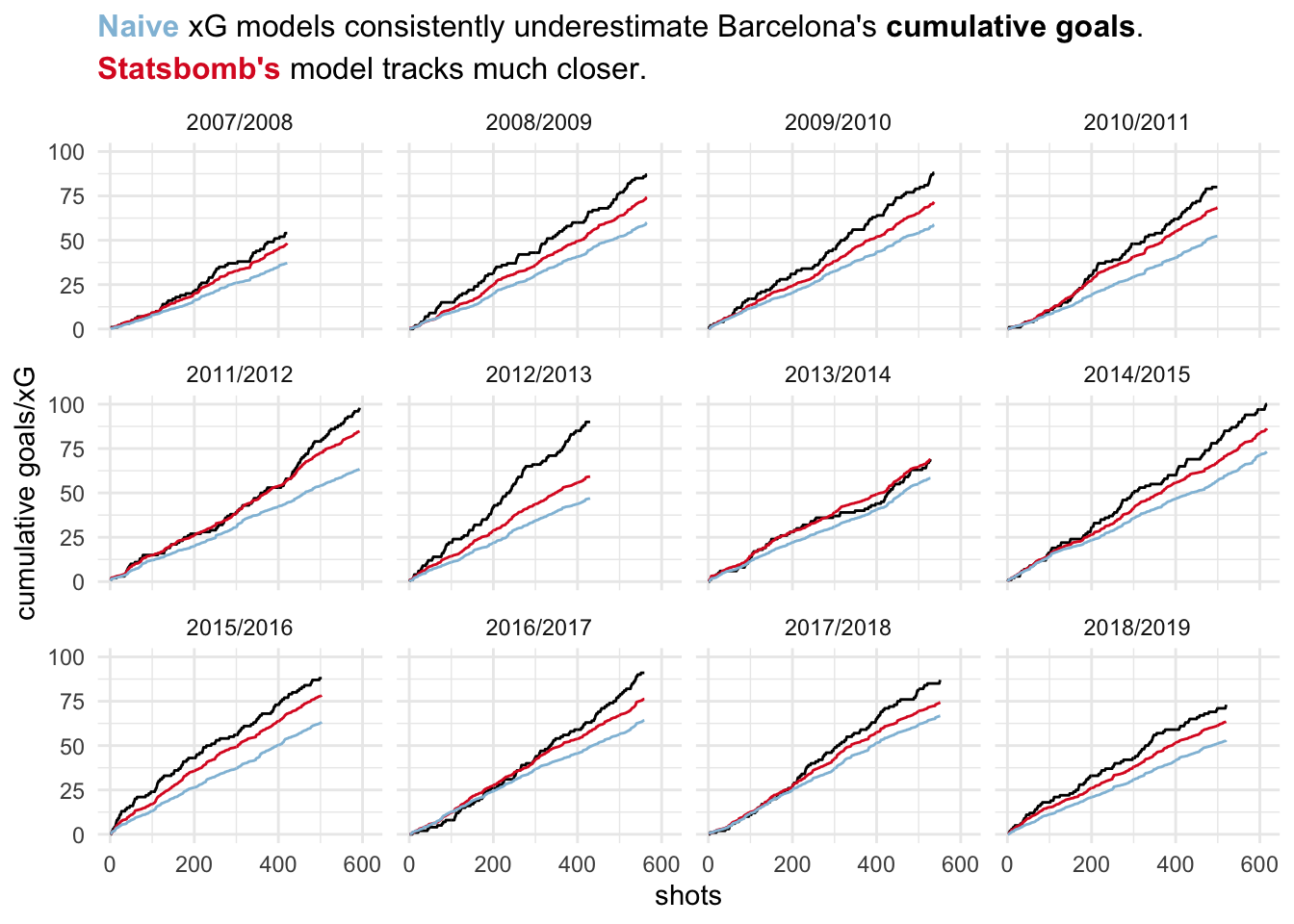
Indeed, while also slightly lower, the Statsbomb model seems to track cumulative goals much better. xG values from the Naive model consistently underestimate goals to a much higher degree.
How does this happen? Let’s assume the only differences between these two models are the additional features that Statsbomb includes. Barcelona may create chances that are above average in terms of these features (18 yard box less congested, goalkeeper in worse positioning, less marginal shots). In the Naive model each shot gets an xG value assigned that is consistent with the average situation across all teams (good or bad) for these situations. This should lead to underestimation (overestimation) of xG for top (bottom) teams.
Let’s next look at the distribution of xG values produced by both models. Remember that they are based on the same sample of shots.
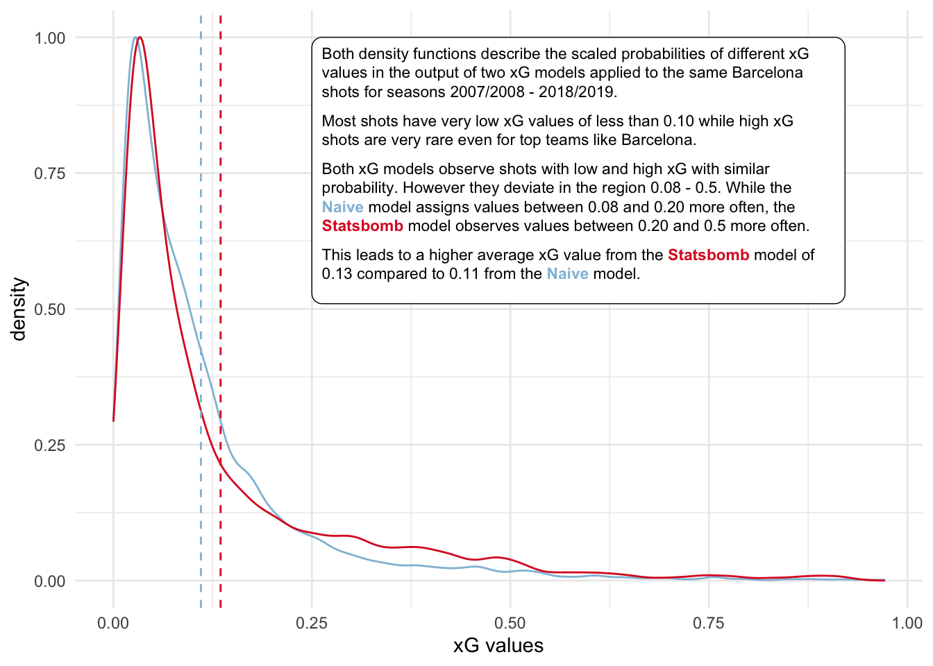
What we have seen so far now is that two different xG models, on a very high level, judge a set of shots quite similarly. But there are difference that do add up over time and larger sample sizes. These differences may be significant or just random. I will next try to investigate what variation we should naturally expect between cumulative goals and xG.
What deviation between goals and xG is abnormal?
Even if we assume that we have a perfect xG model with no estimation error (i.e. the model captures all relevant and repeatable information that influences shot outcome) there will always be residual variance: a shot with true xG of let’s say 0.5 can only either result in a goal or not, i.e. a Bernoulli distributed random variable with parameter equal to xG can only take values of 1 (goal) or 0 (non-goal).
Below in the top chart, I am simulating a large number of cumulative goal paths generated from the same sequence of cumulative xG. Cumulative xG is sampled from a typical distribution like the one we have seen above for Barcelona.
Similar to the Barcelona chart above I show the number of shots on the x-axis and cumulative xG/goals on the y-axis. Possible cumulative goal paths are shown in grey around the red cumulative xG path.
The second chart shows the one-sided, relative variation of the 95% confidence interval around cumulative xG.
This simulation provides us with some useful rules of thumb for the natural variation of cumulative goals around the xG metric. Assuming a perfect model without bias and measurement error, cumulative goals will lie within a +/- 20% range around cumulative xG after one season (with 95% confidence). Variation within this range is therefore not necessarily out- or underperformance of xG, but can simply be driven by the natural variation of Bernoulli random variables.
Similar rules are +/- 50% for 10 games and +/- 33% for half a season.
Note that seasonal data is based on an average of 450 shots which may be quite different for top or poor teams: the ranges will be tighter for teams with high shooting output and wider for low shooting teams.
Thanks to the Central Limit Theorem (CLT) we can make this analysis even more useful by deriving an analytic solution that does not rely on simulations. While the law of large numbers tells us that the sample mean will converge towards the expected value of a sequence of random variables, the CLT provides further details about the variability around the expected value given the sample size and the variance of the individual random variables (the larger the sample size and the smaller the variance, the lower the variance all else equal).
Because our sequence of shots, modeled as Bernoulli random variables, all have different mean (a shot’s xG value) we cannot use the classical CLT which requires independent and identically distributed random variables. Thankfully there is a variant that relaxes the requirement of identical distribution: the Lyapunov CLT.
Click for technical details of the derivation
After checking that the Lyapunov condition holds (it generally does for Bernoulli sequences as long as the limit of the variances is not finite; some more background here) we get that
\(\frac{1}{s_n} \sum_{i=1}^{n} (X_i - \mu_i) {\xrightarrow {d}} N(0,1)\)
This means that the normalized difference of cumulative goals (\(X_i\)) and cumulative xG (\(\mu_i\)) converges in distribution to the standard normal distribution. Therefore
\(P(-1.96 < \frac{1}{s_n} \sum_{i=1}^{n} (X_i - \mu_i) < 1.96) \approx P(-1.96 < N(0,1) < 1.96) \approx 0.95\)
and with a confidence of 95% we have that the difference between cumulative goals and xG lies between
\(P(-1.96s_n < \sum_{i=1}^{n} (X_i - \mu_i) < 1.96s_n)\)
where \(s_n = \sqrt{\sum_{i=1}^{n} \sigma_i^2}\), the square root of the sum of variances of the individual Bernoulli RVs.
Given that xG distributions are fairly similar across teams, I proxy \(\sigma_i^2\) with a random sample of xG data which gives me a value of
\(\sigma_i^2 \approx 0.0878 \approx \frac{1}{12}\)
We combine this with our above result to a new rule of thumb that is a function of shot sample size n
\(P(-1.96 \sqrt{\frac{n}{12}} < \sum_{i=1}^{n} (X_i - \mu_i) < 1.96 \sqrt{\frac{n}{12}})\)
or approximately
\(P(-\sqrt{\frac{n}{3}} < \sum_{i=1}^{n} (X_i - \mu_i) < \sqrt{\frac{n}{3}})\)
For an arbitrary number of shots we now know how much deviation to expect (with 95% confidence) between cumulative xG and goals simple driven by the boolean outcome of shots.
For example, let’s say that we have xG and goals data for 100 teams based on 300 shots each. We expect that for only 5 teams, actual goals deviate from cumulative xG by more than 10 goals (\(\sqrt{\frac{300}{3}} = 10\)) in either direction. Again, this assumes no modeling noise (in reality every model is imperfect and will misjudge shots by some degree).
With this rule of thumb we can now investigate how actual xG models compare to this. Deviations from this rule should give us some insight into their modeling errors.
How do actual xG Models Perform Compared to a Perfect Model?
Given that we now know a bit about how perfect xG models behave in relation to their deviation to cumulative goals over different sample sizes, we can now compare this to the behavior of the Statsbomb model and a Naive model.
The idea is to derive some kind of estimate for how similar they behave to a hypothetical, perfect xG model. For this analysis I will proxy the Naive model again with my own implementation which only relies on location based data (+ some more event flags later).
Data
I am pulling xG data for the Top 5 leagues and three seasons (2017/2018, 2018/2019 and 2019/2020) from Statsbomb (via fbref.com).
This leaves us with 294 team seasons of data for number of shots, cumulative xG (for both Statsbomb and the Naive implementation) and goals. For a perfect model we expect cumulative goals to lie in a range of \(\textstyle{+/- \sqrt{\dfrac{\#shots}{3}}}\) around cumulative xG for around 280 of these seasons (95% of 294). Any deviation from this may indicate the presence of modeling error in the models.
Modeling errors would impact the cumulative xG estimate for each team season and therefore the mid-point of the range. The width of the range solely relies on the variance of a typical xG sample. As we have seen with the data for Barcelona there is not much variation in the distribution of xG values for different models.
The frequency of these outliers should give us an indication of the quality of the model. As we look at the performance of below models we will also include a benchmark non-model that simply uses the average xG (~11.5%) for every shot.
We observe that the Statsbomb model behaves much more similar to the perfect model and that a very simple model is closer to an even simpler No Model. Both the inclusion of location data and having a flag for headers (bodypart) seems to have a sizable impact on accuracy. The build-up play information is less influential. The additional Statsbomb features and their modeling capabilities then deliver again another bump in accuracy.
How should we start thinking about these possible modeling errors? Let’s assume we observe a shot and assign an xG value with A Naive model. Give that we are missing a lot of information (e.g. defender positioning, possibly even bodypart or build-up play) our result will be an average of all similar situations, no matter if the goal is empty or the 6 yard box is congested. Naive models try to overcome this with additional features like flags indicating that a shot occurs after a corner or fast break, but they can hardly be perfect.
Consider the two situations below:
Both shots occur from a relatively similar location in open play. A Naive xG model would assign a similar xG value to both, ignoring the fact that the first shot goes through a congested 6 yard box. A human would possibly assign an xG of 0.4 to the first situation and 0.9 to the second.
Another great source for intuition on how additional features change xG estimates is the Statsbomb article introducing shot impact height.
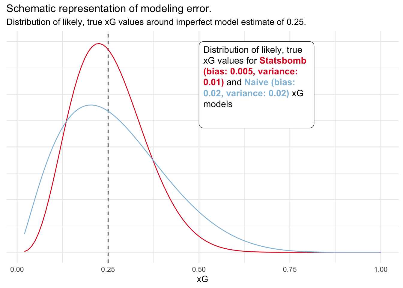
To make this concept a bit clearer we can look at a schematic representation:
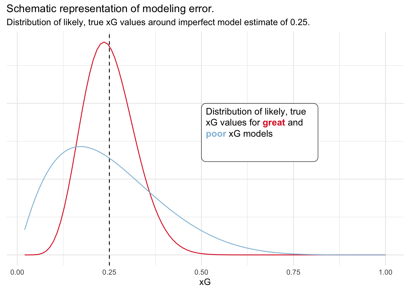
In the above example we have modeled likely, true xG values with the help of a beta distribution with a mean of 0.25. You can think of the beta distribution as similar to the normal distribution but supported only on the interval [0, 1]. It is therefore often visibly not symmetric around the mean, particularly with means close to 0 or 1, or with high variance.
In other words, the range of possible, true xG values for a poor model is wider than for a great model. You can trust the xG estimate from the great model more. We can also turn this thinking around: given a true xG value for a shot, poor models will generate a wider range of model estimates than great models.
In combination with our first simulation we now have a Beta-Bernoulli model: our noisy model xG estimate is beta-distributed around the true xG value and resulting goals are then Bernoulli-distributed and parameterized with these noisy xG values.
Now comes the biggest mental leap in this post: by simulating various mean and variance parameters for the beta distribution (the proxy for model noise) and their subsequent behavior in our first simulation I will try to back out the noise within the Statsbomb and the Naive xG models.
We know that for a perfect xG model, 95% of cumulative goals lie within a certain range around cumulative xG. This drops only slightly for the Statsbomb data (~93%) but more drastic for the Naive modes (~ 79% - 86%). Which noise parameters (shift in the mean or level of variance) are consistent with such a behavior?
In the above table we see that Statsbomb’s model is likely unbiased. Its behavior is most consistent with minimal bias and variance between 0.005 and 0.01. The Naive model likely contains some form of bias (~0.02) and some variance. We can see below how this would look visualized for an example xG value of 0.25. We can see that the Statsbomb model gives us larger confidence in its estimate. Potential true xG values are narrowly distributed around the estimate.
A few points of caution now. The above results are based on quite a few assumptions and the above parameter estimates can only be treated as indicative. We are assuming that true xG values are beta-distributed around the xG estimate. This may vary from situation to situation but on average seems to be a good choice as it resembles the unconditional distribution of xG values.
Another modeling choice is the application of the bias in the above simulation. Given that xG models are calibrated with the goal of not showing any bias across many teams, seasons and leagues we need to be a bit clever to not introduce any overall bias.
Similar to our initial idea of potential bias for top and bottom team, we will apply the bias only to a random 25% of sample in positive form and another 25% in negative form. Therefore we are able to introduce modeling noise without introducing overall bias to the model. The choice of 25% is arbitrary and will likely impact the overall bias estimate we find consistent with our observed data (In the second table we observe how estimated values change when only applying the bias to top/bottom 10%).
Even with the above uncertainties I think this is a very useful framework to think about relative quality of xG models.
Do Naive xG Models underestimate Expected Goals for Top Teams?
We now have good indications that Naive xG models are biased for a certain subset of teams. We can now go back to our original question: is there systematic bias towards teams with high or low shooting volume?
To answer this, let’s try to find bias in the types of teams who’s seasons do not fall in the 95% confidence interval.
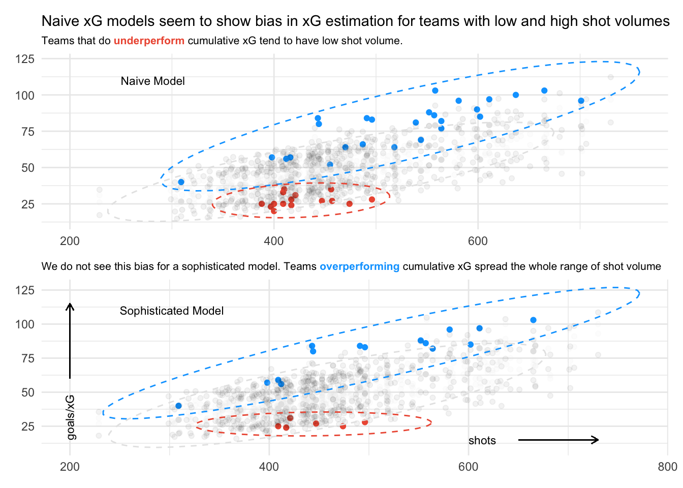
Below I am plotting cumulative goals vs shots from our 294 team seasons. I am only highlighting goal data that lies outside the 95% confidence intervals for both Naive (I am using the version with most features; including body part and build-up play) and Statsbomb xG estimates. Cumulative goals that lie above the interval are highlighted blue, goals below the interval are highlighted red.
As expected we see many more data points highlighted for the Naive data than for Statsbomb’s. In both cases we see that xG gets overestimated for teams on the side of lower shot volume (red data). I assumed that xG underestimation would only happen for teams with high shot volume, but we see it happen for teams across the full range. Extreme data seems to be clustered a bit more for teams with higher shot volume, but the evidence seems pretty weak.
Sensitivity to measure of “top”
The number of taken shots over a season is a pretty vague definition of “top team”. To really investigate this relationship let’s look at another definition of team quality: Elo rating. Because we do not want to use a definition that relies on the coincidental performance of a team to the xG data we have, we use Elo ratings in the summer prior to a season’s xG data.
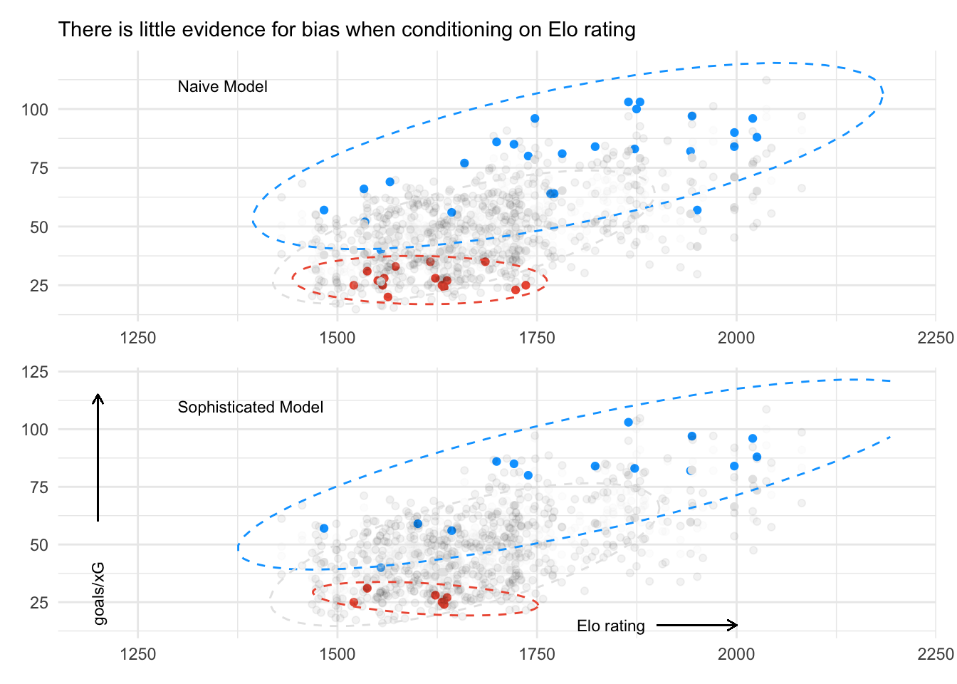
The analysis is pretty similar when conditioning on Elo rating instead of shot volume. In this case, shot volume may be a pretty good proxy for team quality.
Overall however, there seems to be relatively weak evidence for systematic over/underestimation of xG depending on team quality.
Comparison to David Sumpter’s (Soccermatics) Rules
A lot of the things I have looked at overlap with David Sumpter’s analysis in Should you write about real goals or expected goals?. My view is that my results are consistent with his findings but offer a more granular view of the variability of goals around expected goals by relating it to the number of shots not games. I also highlight the difference the quality of an xG model makes.
David answers two main questions: With what sample size does it make sense to start looking at xG values and when should you prefer actual goals over xG?
In order to answer these questions I will initially deviate from David’s guidance to again assume there is a hypothetical, perfect xG model who’s output is superior even to goals at any sample size.
Next I will measure noise to this hypothetical model for actual goals, a sophisticated model and a naive model. These two models are again proxied by the modeling errors I derived from Statsbomb and Naive data.
Initially, with very low sample size, we observe that both xG models have lower errors than goals. This makes intuitive sense given that goals can only take values between 0 and 1 and we need some time for the law of large numbers to kick in.
It certainly does not make sense to blindly trust xG values accrued over just one game. The one-sided width of the confidence interval for xG models lies between 33% and 60%, i.e. if your naive model provides you with cumulative xG of 1.0, true xG may very well lie anywhere between 0.4 and 1.6.
After 5 games the one-sided error drops to 20% to 35% which is definitely more useful.
Goals pass a naive xG model in accuracy somewhere between 10 games and half a season, similar to what David outlines in his analysis. Our naive xG model also seems to stop converging after this point. This is caused by its bias that systematically keeps cumulative xG values from converging to true xG for some teams.
If our modeling for the sophisticated xG model is correct, it fairs better than goals for quite some time. The error for goals only really gets comparable after two seasons.
This really illustrates the power of a very good xG model. It allows you to act on your data earlier and provides you unique insights while other analysts have to wait until goals converge to a similar error rate.
Summary
I have introduced a framework to roughly quantify the varying quality of xG models. By comparing their behavior in analyzing shots from almost 300 team seasons to a hypothetical, true xG model I find that the more sophisticated Statsbomb model outperforms a simpler model.
I further investigate if any of the models show a bias in analyzing shots of teams with either high or low shot volume. I find that naive xG models tend to underestimate expected goals for teams with high shot volume and overestimate xG for teams with low shot volume. I do not find this effect for the more sophisticated Statsbomb model that includes additional features like shot freeze frames, goalkeeper positioning and shot impact height.
This effect may by driven by a systematic underestimation (overestimation) of xG for top (bottom) teams, but when conditioning on another metric of team quality (Elo ranking) I do not find this bias in either naive or sophisticated models.
A possible explanation for these observations would be that top teams with higher shot volume are more careful about choosing their shooting opportunities and when in doubt (congested 18 yard box or awkward shot height) recycle the ball instead of pulling the trigger. Another explanation could be superior finishing ability of top players. The missing evidence when conditioning on Elo ranking however call my initial intuition into question.
Along the way I also find some useful rules of thumb to help judge if goals actually significantly outperform cumulative xG or if they are within an interval consistent with the expected variation of Bernoulli random variables for a given sample size.
For a given cumulative xG value x based on n shots, we expect the resulting goal tally to lie within the interval \([x - \sqrt{\frac{n}{3}}, x + \sqrt{\frac{n}{3}}]\). As an example: for a sample size of 300 shots this range is 20 goals wide.
For a typical team (based on 450 shots per season of typical shot quality) goals vary 50% around cumulative xG after 10 games, 33% after half a season and 25% after a full season. These values are of course only rough guidelines.
The above two rules seem to be consistent with David Sumpter’s analysis in Should you write about real goals or expected goals?
Update
Earlier versions of this post compared Statsbomb and Understat xG data. I have since switched to comparing Statsbomb data to my own implementation of a Naive xG model. This allows me to judge more granularly the improvements achieved when adding more features (like build-up play) over location data.