xG Model - Design and Implementation with R Tidymodels
I have recently gone through the Google Machine Learning crash course and was looking for a project to apply these skills to. Coincidentally, it is also not that long ago that tidymodels has gained some traction (at least in my twitter feed) and I am keen to try it out.
Of course an Expected Goals-model is a great excuse to combine the two items above. It is relatively easy to set up, readers of this blog will not need a lengthy introduction to the thought process behind it and the feature set used to explain the probability of shots leading to goal is very intuitive.
Of course, there has already been written so much about xG-models and I am also certainly not the first to implement it in R. So let me give a quick overview about the best writing I have seen to then give some thoughts about what I hope to add to the discussion with this post.
- David Sumpter’s Friends-of-Tracking initiative on Youtube
- The DTAI Sports Analytics Lab of KU Kleuven has an outstanding blog focused on machine learning techniques in soccer analytics
- American Soccer Analysis consistently publishes great and detailed articles on data-driven aspects of the game
I am missing the earlier history of the process that is the creation of the expected goals metric, but it is not my goal to come up with this timeline, but to highlight the articles and videos I found most useful.
To avoid being redundant I will try to outline how to implement xG-models in a modern tidy R framework via tidymodels, to evaluate the fit of the model through methods I learned through the Google’s ML course and to finally contrast what xG-models are and aren’t good at. In this first post I will show how to implement a simple xG-model.
Let’s start by loading the necessary libraries and helper functions.
library(dbplyr) # database access
library(DBI) # database access
library(tidyverse) # dataframe manipulation
library(tidymodels) # data processing and modeling

source("../data/pitch_plots.r") # helper function to plot the pitch
You can see our initial dataset below. This is bare-bones event data represented in a wide dataframe with each row representing one shot. Notably we do not have any information on the shooter, the teams or the match. For our initial model we will actually only use the three left most columns which hold information on the location and the outcome of each shot. These are all open-play shots, meaning that I made sure to filter out any headers, penalties, shots after corners or from free kicks.
## # A tibble: 51,981 x 12
##    location_x location_y is_goal big_chance header from_corner from_fk direct_fk
##         <dbl>      <dbl>   <dbl>      <dbl>  <dbl>       <dbl>   <dbl>     <dbl>
##  1       74.8       64.5       0          0      0           0       0         0
##  2       87.5       61.5       0          1      0           0       0         0
##  3       78.2       72.3       1          0      0           0       0         0
##  4       80.5       44.7       0          0      0           0       0         0
##  5       91.3       59         1          1      0           0       0         0
##  6       67.4       36.3       0          0      0           0       0         0
##  7       79.5       33         0          0      0           0       0         0
##  8       78.6       51.1       0          0      0           0       0         0
##  9       79.5       41.5       0          0      0           0       0         0
## 10       70.8       55.7       0          0      0           0       0         0
## # … with 51,971 more rows, and 4 more variables: penalty <dbl>, assisted <dbl>,
## #   intentional_assist <dbl>, fast_break <dbl>
Next I start with the feature engineering step. While you can certainly use the raw position information for predicting the xG-value of a shot, we follow the Friends-of-Tracking (FoT) tutorial by creating a distance and an angle metric.
distance <- function(x_pos, y_pos){
  x_meters <- 95.4
  y_meters <- 76.25

  x_shift <- (100 - x_pos)*x_meters/100
  y_shift <- abs(50 - y_pos)*y_meters/100

  distance <- sqrt(x_shift*x_shift + y_shift*y_shift)
}

goal_angle <- function(x_pos, y_pos){
  x_meters <- 95.4
  y_meters <- 76.25

  x_shift <- (100 - x_pos)*x_meters/100
  y_shift <- (50 - y_pos)*y_meters/100

  angle <- atan((7.32*x_shift)/(x_shift*x_shift + y_shift*y_shift - (7.32/2)*(7.32/2)))
  angle <- ifelse(angle < 0, angle + pi, angle)

  angle_degrees <- angle*180/pi
}

shots_ext <- shots_ext %>%
  rowwise() %>%
  mutate(distance = distance(location_x, location_y)) %>% # distance from goal mid-point
  mutate(angle = goal_angle(location_x, location_y)) %>% # based on available goal mouth
  ungroup()
In the next step we are making use of the tidymodels package the first time. Our goal is to shuffle our shot data and to split it into a training and a testing set. The shuffling ensures that we eliminate any unwanted patterns in the data. The shots could potentially be sorted by distance to goal in a way that the training data only contains shots outside of the 6 yard box. This would likely lead to suboptimal results when we apply our fitted model to real life data.
Two more small points to highlight: - In the first line we format the shot outcome from numeric to factor. This is necessary as the label for the logistic regressions needs to be a categorical variable. - When we define our recipe we first include the raw location data (location_x and location_y) in our formula, to then give them the role of “ID”. This lets us keep the location information in our dataframe without using them as predictors in our regression.
I do not particularly like this design principle but it enables us to later compare our xG estimation directly to the location of the shot.
shots_ext$is_goal <- factor(shots_ext$is_goal, levels = c("1", "0"))

set.seed(seed = 1972)

train_test_split <- initial_split(data = shots_ext, prop = 0.80)

train_data <- train_test_split %>% training()
test_data  <- train_test_split %>% testing()

xg_recipe <-
  recipe(is_goal ~ distance + angle + location_x + location_y, data = train_data) %>%
  update_role(location_x, location_y, new_role = "ID")

summary(xg_recipe)
## # A tibble: 5 x 4
## variable type role source
## <chr> <chr> <chr> <chr>
## 1 distance numeric predictor original
## 2 angle numeric predictor original
## 3 location_x numeric ID original
## 4 location_y numeric ID original
## 5 is_goal nominal outcome originalNext we define our model to then combine it with our recipe to a model workflow. Our model is a simple logistic regression executed by the glm engine.
At this point you have the flexibility to change the engine to other regression/machine learning libraries like keras. The great advantage of tidymodels is that you can do so without changing anything else in your code. The package deals with different conventions and formats in the background.
model <- logistic_reg() %>%
  set_engine("glm")

xg_wflow <-
  workflow() %>%
  add_model(model) %>%
  add_recipe(xg_recipe)

xg_wflow
## ══ Workflow ═══════════════════════════════════════════════════════════════════════════════════════════════════════════════════════════════════════════
## Preprocessor: Recipe
## Model: logistic_reg()
##
## ── Preprocessor ───────────────────────────────────────────────────────────────────────────────────────────────────────────────────────────────────────
## 0 Recipe Steps
##
## ── Model ──────────────────────────────────────────────────────────────────────────────────────────────────────────────────────────────────────────────
## Logistic Regression Model Specification (classification)
##
## Computational engine: glmWe are now ready to fit our model and to inspect the estimated parameters and their significance.
Let’s first think about which sign the weights of our two predictor variables should have. For that we should first recall the sigmoid function used in the logistic regression
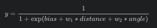
This function ensures that our model’s prediction will be between 0 and 1.
The longer the distance of the shot from goal, the lower the xG value should be. We therefore expect a positive weight for this predictor (larger argument for the exponential and therefore larger denominator).
The larger the angle of the shot, the higher the xG value should be. We therefore expect a negative weight for this predictor (smaller argument for the exponential and therefore smaller denominator).
We see both of these expectations satisfied in the below output. Additionally we also observe that all of our estimation are statistically significant.
xg_fit <-
  xg_wflow %>%
  fit(data = train_data)

xg_fit %>%
  pull_workflow_fit() %>%
  tidy()
## # A tibble: 3 x 5
## term estimate std.error statistic p.value
## <chr> <dbl> <dbl> <dbl> <dbl>
## 1 (Intercept) 0.435 0.108 4.02 5.84e- 5
## 2 distance 0.139 0.00473 29.4 1.25e-189
## 3 angle -0.0205 0.00161 -12.8 2.01e- 37Let’s go through a quick example to get an even better intuition for the model. Think about what the xG value should be for a shot from the penalty spot. Note that these are not actual penalties with unobstructed paths but open-play shots from around the penalty spot.
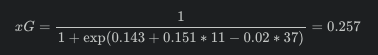
Next we want to overlay a pitch plot with the output of our xG-model. For this we first need to create a dataframe of artificial shot data spanning the whole area of the pitch (or half pitch). Again we create our predictor variables and call the predict-function on this dataframe. We end up with a column named xG that contains an xG-estimate for each of these (artificial) shots.
artificial_shots <- crossing(location_x = seq(50, 100, by = 0.5), location_y = seq(0, 100, by = 0.5)) %>%
  mutate(distance = distance(location_x, location_y)) %>% # distance from goal mid-point
  mutate(angle = goal_angle(location_x, location_y)) # angle based on available goal mouth

data_to_plot <- predict(xg_fit, artificial_shots, type = "prob") %>%
  bind_cols(artificial_shots) %>%
  rename("xG" = ".pred_1")
Let’s plot:
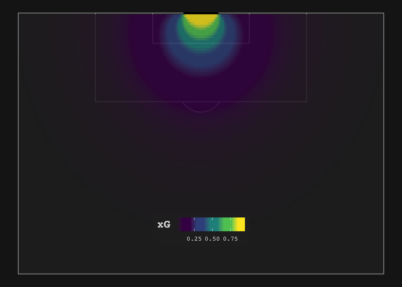
This looks reasonable. We see the well-known circle-like shape radiating out from the goal line. The highest value is shown centrally in front of goal. xG values decrease further out and importantly decrease at with smaller angles. The xG estimates also make sense: we have already seen that an open-play shot from around the penalty spot results in a xG-Value of 0.25; centrally, just outside the 18 yard box we see a value of around 9% which also matches my expectation.
In the next post I will try to evaluate some goodness-of-fit measures for this model to contrast applications that are suited for an xG-model and those that are not.
comments powered by Disqus