xG Model - Accuracy and Goodness-Of-Fit
In the first part of this series we constructed a simple expected Goals-model, solely relying on two predictors: the distance and angle from goal for each shot.
As a reminder see below the visualization of our xG-estimates from the first part of this series:
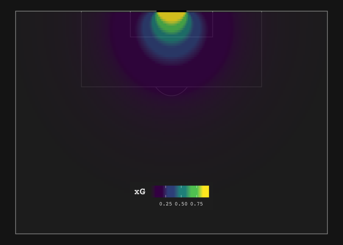
Our model passed the eye test, i.e. it maps shot locations to xG-values that make intuitive sense to us.
In this post we want to evaluate the quality of this model more formally with tidymodels’ yardstick package.
Our modeling problem is not much different to the classic machine learning application of classifying spam and non-spam emails. With an xG-model we try to predict the outcome of a shot based on properties associated with it (location, build-up, body part); for a spam-classification model you try predict if the email is unwanted spam based on properties associated with the email (sender, subject, certain words, language, time sent).
Even though we’ll see that xG modeling is vastly harder than spam classification I will go through the common steps of evaluating the goodness-of-fit for classification models.
Accuracy
As a first step we can compute the accuracy of our model, i.e. how often does our model classify a shot correctly as a goal or non-goal. For this we need to make a decisions about the threshold we want to use for this prediction.
For which xG-values do we want to make the prediction that a shot will likely result in a goal? An obvious starting point would be 0.5. This may initially sound strict as for our model this will only predict goals for shots within the 6 yard box (you can see this in the above plot), but choosing a value lower is like betting against an unfair coin. This would also repeat the mistake of pundits predicting that any shot within the 18 yard box is a sitter.
In the below chunk we again use our fitted model to generate xG-values to then classify them as goal or non-goal in a column is_goal_pred. We then use yardstick’s metrics function which provides us with value for accuracy.
xg_pred <- predict(xg_fit, test_data, type = "prob") %>%
  bind_cols(test_data) %>%
  rename("xG" = ".pred_1") %>%
  mutate(is_goal_pred = factor(if_else(xG > 0.5, 1, 0), levels = c("1", "0")))

xg_pred %>%
  metrics(truth = is_goal, is_goal_pred) %>%
  select(-.estimator) %>%
  filter(.metric == "accuracy")
## # A tibble: 1 x 2
## .metric .estimate
## <chr> <dbl>
## 1 accuracy 0.905An accuracy of 90.5% sounds pretty good at first, but we need to bring this into the context of our data. The shot/goal data is a highly class-imbalanced data set, meaning that there is a significant disparity between the number of positive (goal) and negative labels (no goal). If 90.5% of all shots do not results in a goal our model is no better than a model with no explanatory power at all but always predicting no goal.
Confusion Matrix
To shine some more light on this question let’s look at the confusion matrix of our model predictions. In a 2-by-2 matrix it aggregates events based on their true outcomes and the model’s predictions. And indeed, of our 10396 shots in our test data, 9373 or 90.2% did not result in a goal. Solely judged on this metric our model is not better than no model at all, i.e. blindly always predicting no goal.
xg_pred %>%
  conf_mat(truth = is_goal, is_goal_pred) %>%
  pluck(1) %>%
  as_tibble() %>%
  ggplot(aes(Prediction, Truth, alpha = n)) +
  geom_tile(show.legend = FALSE) +
  geom_text(aes(label = n), colour = "white", alpha = 1, size = 8)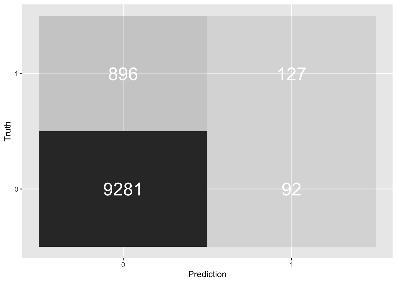
Precision and Recall
So accuracy alone does not seem to give us a good sense of how good our model is. Let’s look at precision (What proportion of positive identifications was actually correct?) and recall (What proportion of actual positives was identified correctly?). You may have already noticed in the confusion matrix that we have a problem here: out of the 1023 goals we only predicted 127 correctly (12% recall) and out of our 219 goal predictions only 58% were correct.
tibble(
  "precision" =
     precision(xg_pred, is_goal, is_goal_pred) %>%
     select(.estimate),
  "recall" =
     recall(xg_pred, is_goal, is_goal_pred) %>%
     select(.estimate)
) %>%
  unnest(cols = c(precision, recall))
## # A tibble: 1 x 2
## precision recall
## <dbl> <dbl>
## 1 0.580 0.124Skill vs Luck
It becomes clear that our xG-model is not very good at deciding if individual shots result in goals.
After thinking about all the information we do not capture this should not be surprising. At this point we can categorize the missing information in three categories:
A) Information we can proxy with simple event data:
- shot location
- body part (head or foot)
- build-up play (penalty, cross, fast break, …)
- …
B) Information for which we need more sophisticated (event or tracking) data:
- position of goalkeeper
- position of defenders
- footedness of shooter
- velocity and direction of defenders
- …
C) Information that is currently unobservable or we will never be able to reliably collect:
- exact angle and location of body part striking the ball
- reaction time of goalkeeper
- wind speed
- air pressure of the ball
- … (you get the idea and you can get very creative here)
We may call a xG-model that only uses the first category of data naive and one that uses both the first and second category sophisticated. A hypothetical model that uses all three categories of information is simply the goal tally. It will always correctly predict if a shot results in a goal or not.
Another way to look at this is to classify categories A and B as repeatable properties of a shot or skill and the third category as non-repeatable or luck. One goal of analytics and data gathering is to expand category B at the cost of category C. Identifying repeatable skills will allow you to improve your xG-model and make better decisions based of it.
Statsbomb has recently published a great post on this when they announced a new feature for their xG-model: shot impact height. In a range of examples they show how large the impact of this new feature can be on their xG-estimates. Essentially they have taken a feature from category C and moved it to category B.
We approach the limit of xG-modeling when thinking about penalties. The static set-up of penalties allows us to have all possible information form categories A and B available (we always know the shot height, position of the goal keeper and defenders, the shot is taken with the shooter’s strong foot, …). Even then we can do no better than to assign a fixed value of 0.75 to penalties.
The difference between the xG-Value for an open-play shot around the penalty spot and the xG-value for a penalty tells another interesting story and allows us to estimate the magnitude of the impact of features in category B. The average xG for a shot in this location is 0.25 but there are many shots with significantly lower and higher true xG.
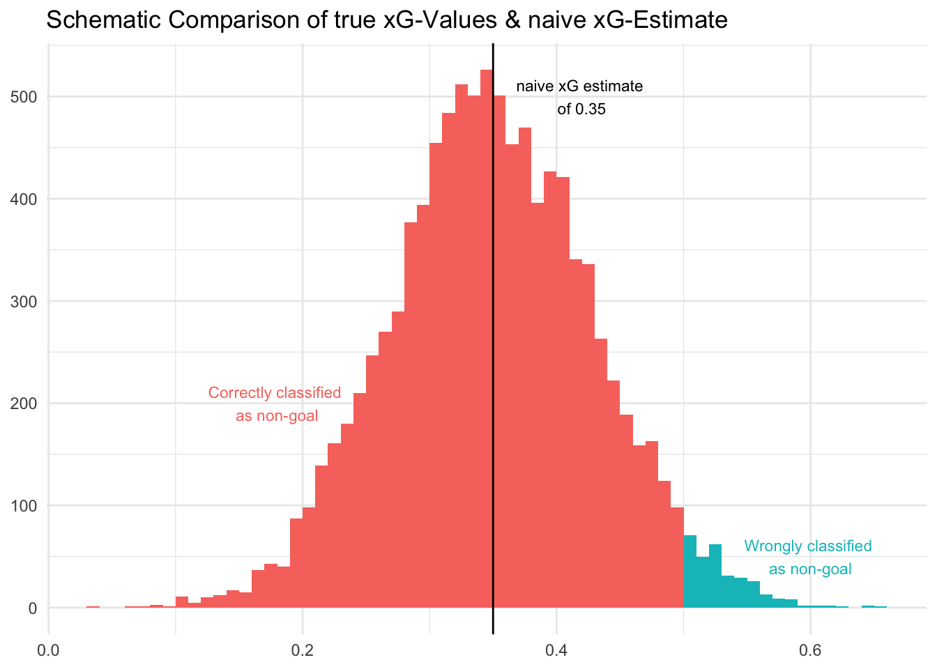
This also explains why our model underestimates the percentage of shots resulting in goal in the above confusion matrix. Our threshold of 0.5 classifies all of the shots with a naive xG of 0.35 as non-goal while quite a few of them have a true xG-value of higher than 0.5. The reverse is true for shots with naive xG of smaller than 0.5 but there are simply many more shots with low xG (below 0.25 or 0.10) which then leads to this bias in estimation.
In a statistical sense, by improving our model, we reduce the variance around a hypothetical, true xG-value so that our imperfect estimates converge faster to their true value. This higher confidence in your xG estimate will be useful to better judge a player’s goal contribution, a team’s form or to identify promising build-up patterns (e.g. pull-backs).
Both naive xG-estimates and actual goal tallies can be thought of as fluctuating around a hypothetical, true xG-value. One difference is that actual goals are certain to ultimately converge (with large sample size) to this true xG-value. This is the definition of luck, the unrepeatable variance around a true value. To the contrary, omitted explanatory variables in naive xG-models can lead to divergence between cumulative xG-estimates and cumulative goals: people call this “breaking xG” (something that is frequently associated with Lucien Favre).
In theory, breaking xG is not very hard to do and for many elite teams it comes naturally. Simply improving shot locations will not do it as all spatial information is incorporated even in the simplest xG models. But repeatably taking above-average quality shots (keeping the location constant) will over time break xG as long as the improved feature of the shot is currently not captured by the xG model.
Let’s move to things that our model is actually decent at. We know that xG-models get things on average:
Modeling Bias
While our model has problems determining the number of goals based on boolean predictions (goal/non-goal) with our threshold of 0.5, the average xG is in line with our expectation that around 10 shots are taken per goal.
And this is what we really care about for most applications of the xG framework. One of the few cases for which we may want to convert xG-values to actual goals are expected Points or win probabilities based on xG. For this you can usually rely on simulation techniques.
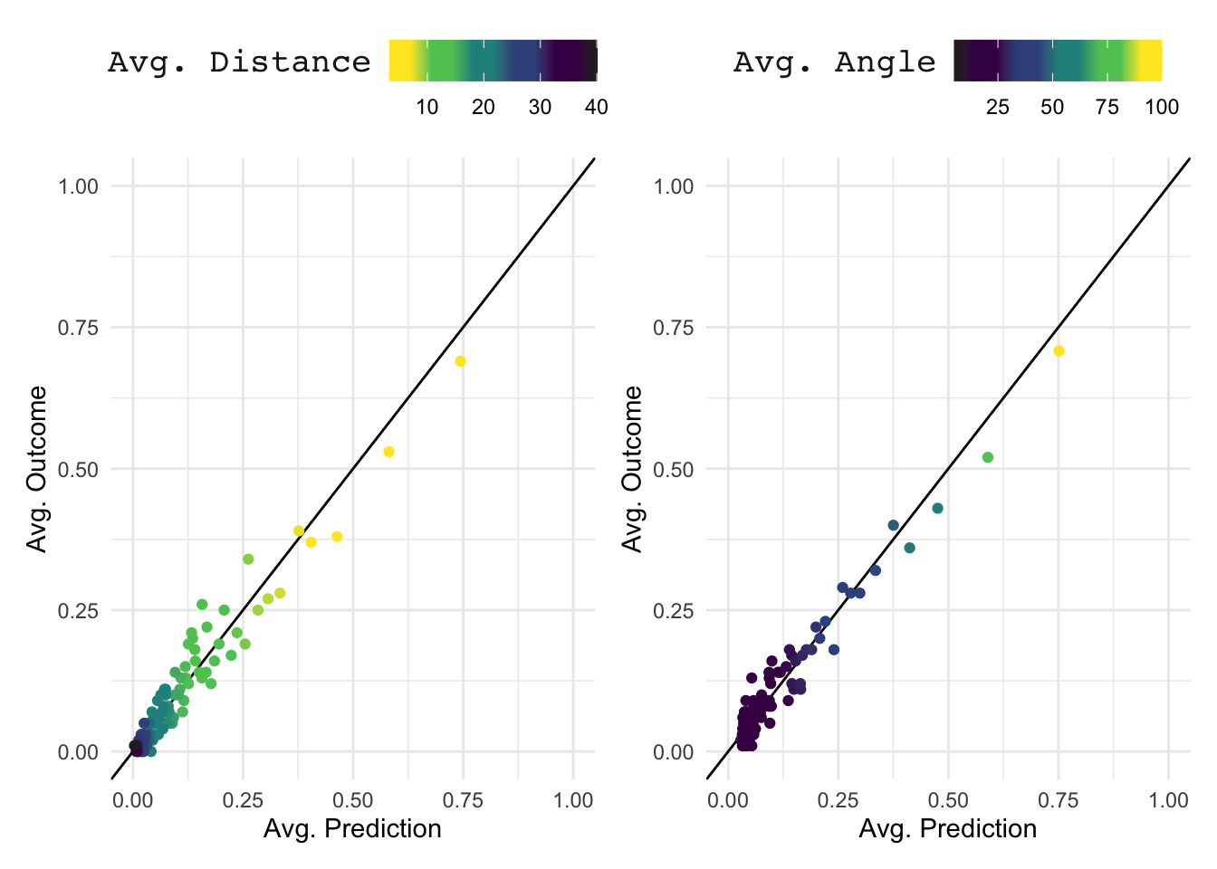
To determine any modeling bias we need to assess the model predictions across a larger subset so that the law of large number can work its magic. For the below chart we group shots in sets of 100 to then compute average goals and average xG per shot.
To investigate the impact of both our features we also sort the initial data set separately by distance and angle (e.g. the 100 shots with the largest distance are all part of the same subset). We want to avoid that our model only works for shots outside the 18 yard box or only for shots centrally in front of goal. Blind spots like this may be masked by the wider data set if only few shots have certain features.
In the below chart each dot represents a set of 100 shots. Distance and angle are represented through the fill colors. Not all dots lie on the ideal 45 degree line, but more importantly we do not see any bias driven by certain distances or angles.
ROC Curve
Another way to assess the goodness-of-fit of our model is a ROC curve (receiver operating characteristic curve). It highlights the trade-off between the true positive-rate (y-axis) and the false positive-rate for many different threshold values. For an ideal model we would see the curve stretch all the way to the top left of the quadrant, but any curve left of the dashed line is better than a random model. The area under the curve can be interpreted as the probability that the model ranks a random positive example more highly than a random negative example.
We can again use the yardstick package to produce the below:
xg_pred %>%
  roc_curve(truth = is_goal, xG) %>%
  autoplot()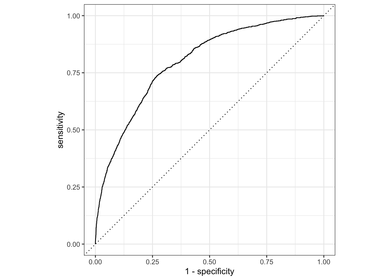
Summary
In this post we have explored tools from tidymodels’ yardstick package to assess the goodness-of-fit of our naive xG-model solely relying on shot location.
We have build intuition for the fact that xG-models are not good at predicting the (boolean) outcome of individual shots (or group of shots for that matter) by highlighting the large number of features not included in simple xG-models.
We have shown how xG-estimates for group of shots are still useful on average and how by improving our xG-model we should be able to reduce the variance of our xG-estimates so they converge quicker to a hypothetical, true xG-value.
In a next post I will see how much of an improvement in the above metrics we can achieve by incorporating some additional metrics into the model. I will also show how hard it is to make any statement about finishing skills of individual players and we will check if Cristiano Ronaldo is a superior penalty taker.
- More on the ROC curve