First Look at SkillCorner's Open Source Tracking Dataset
A couple of weeks ago another great dataset was made available to the soccer analytics community. In collaboration with Friends-of-Tracking the data provider SkillCorner open-sourced tracking data for nine matches across the Top5 leagues.
Here is the link of the 9 matches of broadcast tracking data, we're open sourcing today:https://t.co/4CnxCO1EAC
— SkillCorner (@SkillCorner) October 8, 2020
We'll open source soon some tooling to help visualizing the data, computing derivatives or synchronizing the data with event data.
SkillCorner’s data is a little different from the usual tracking data in that they are emphasizing broader coverage across as many leagues as possible over 100% accuracy. Their so-called broadcast tracking data is automatically generated from TV footage with no or little postprocessing. Conventional tracking data relies on multiple cameras and is much more expensive to generate, but will ensure that all 22 players are always in the frame.
One of the downsides of broadcasting footage as a source is therefore that it suffers from noise in the form of replays and close-up zooms. In this post I will try to introduce the format of the data and some ways to work around its quirks.
Let’s start with loading the necessary libraries and with sourcing data for the 4:0 win of Bayern Munich against Borussia Dortmund in November 2019 from SkillCorner’s GitHub repository (ID 2417). The time frame from 45:50 to 46:10 covers Serge Gnabry’s 2:0 goal assisted by Thomas Müller.
I am also sourcing a custom pitch plotting function from one of my repositories. The format for the start and end time is HH:MM.(1/10th sec)
library(tidyverse) # Data manipulation
library(jsonlite) # Loading json files
library(gganimate) # Animation of plots
library(gridExtra) # Needed for adding tables to plot
library(cowplot) # Needed for adding images on plot

# This is a simple pitch plotting function that expects data formatted to a 105x86m pitch
source("https://raw.githubusercontent.com/larsmaurath/keine-mathematik/master/content/data/pitch_plot.R")


# Start and end time of the frames we want to plot
start_time <- "45:50.0"
end_time <- "46:10.0"
half <- 2 # If the times are close to 45min, we need to specify which half we mean


# Load meta data and actual tracking data
meta <- fromJSON("https://raw.githubusercontent.com/SkillCorner/opendata/master/data/matches/2417/match_data.json")

players <- meta[["players"]] %>%
  select(trackable_object, last_name, team_id, number)

tracking <- fromJSON("https://raw.githubusercontent.com/SkillCorner/opendata/master/data/matches/2417/structured_data.json") %>%
  filter(time > start_time & time < end_time & period == half)
Tracking data is stored as one row per frame with the actual x/y-coordinates by object stored in dataframes in the data column. We therefore loop through each row to concatenate the location information into a new dataframe called coordinates.
If the broadcast feed does not show a clear of view of the action or a review the returned dataframe will be empty. In this case we simply fill forward the information from the previouse dataframe, but indicate in a new column is_broadcast that this is not live information.
# We are looping through frames and concatenate tracking data.
# If tracking data is not available we fill forward the previous
# frame and flag it as 'not in broadcast'.

coordinates <- c()

for (i in seq(1, nrow(tracking))) {
    frame_df <- tracking[i, ]$data[[1]]

    if(!nrow(frame_df)){
      frame_df <- prev_frame_df %>%
        mutate(in_broadcast = FALSE)
    } else{
      frame_df <- frame_df %>%
        mutate(in_broadcast = TRUE)

      prev_frame_df <- frame_df
    }

    frame_df <- frame_df %>%
      mutate(frame = tracking[i, ]$frame) %>%
      mutate(time = tracking[i, ]$time)

    coordinates <- bind_rows(coordinates, frame_df)
}
One way to deal with the mentioned gaps in the data is to linearly interpolate the x/y-coordinates. For this we assume that all players and the ball move on the shortest path at constant speed to their new location (i.e. where they reappear once the footage is back live or zoomed out). Of course this assumption can be very wrong, but should be OK for short gaps.
# Below code interpolates linearly between locations
# for periods in which we have missing tracking data

coordinates <- coordinates %>%
  group_by(trackable_object ) %>%
  mutate(x_start_value = ifelse(in_broadcast, x, NA)) %>%
  mutate(x_end_value = ifelse(in_broadcast, x, NA)) %>%
  mutate(x_start_frame = ifelse(in_broadcast, frame, NA)) %>%
  mutate(x_end_frame = ifelse(in_broadcast, frame, NA)) %>%
  fill(x_start_value, .direction = c("down")) %>%
  fill(x_end_value, .direction = c("up")) %>%
  fill(x_start_frame, .direction = c("down")) %>%
  fill(x_end_frame, .direction = c("up")) %>%
  mutate(y_start_value = ifelse(in_broadcast, y, NA)) %>%
  mutate(y_end_value = ifelse(in_broadcast, y, NA)) %>%
  mutate(y_start_frame = ifelse(in_broadcast, frame, NA)) %>%
  mutate(y_end_frame = ifelse(in_broadcast, frame, NA)) %>%
  fill(y_start_value, .direction = c("down")) %>%
  fill(y_end_value, .direction = c("up")) %>%
  fill(y_start_frame, .direction = c("down")) %>%
  fill(y_end_frame, .direction = c("up")) %>%
  ungroup() %>%
  filter(!is.na(x_end_value))

coordinates_int <- coordinates %>%
  rowwise() %>%
  mutate(x = ifelse(in_broadcast, x, approx(x = c(x_start_frame, x_end_frame),
                                            y = c(x_start_value, x_end_value),
                                            xout = frame,
                                            method = "linear")$y)) %>%
  mutate(y = ifelse(in_broadcast, y, approx(x = c(y_start_frame, y_end_frame),
                                            y = c(y_start_value, y_end_value),
                                            xout = frame,
                                            method = "linear")$y)) %>%
  ungroup()
To plot the tracking data in an animation we first want to standardize the coordinates to a 105m x 68m norm to then use our plotting function. gganimate will then take care of the rest. Its function transition_time specifies which dataframe column holds the frame information. We plot players and ball separately to ensure that the ball is always visible (i.e. on top).
coordinates_int <- coordinates_int %>%
  left_join(players, by = "trackable_object" ) %>%
  mutate(team_id = ifelse(trackable_object == 55, 0, team_id)) %>%
  mutate(time = as.POSIXct(time, format="%M:%OS")) %>%
  mutate(x = x + 52.5) %>% # necessary conversion for pitch plot function
  mutate(y = y + 34) %>% # necessary conversion for pitch plot function
  filter(!is.na(team_id))

p <- plot_pitch(theme = "dark") +
  geom_point(data = coordinates_int %>% filter(trackable_object != 55),
             aes(x = x,
                 y = y,
                 color = factor(team_id),
                 size = factor(team_id),
                 group = time,
                 alpha = in_broadcast)) +
  geom_text(data = coordinates_int,
            aes(x = x, y = y, label = number, group = time),
            size = 3,
            colour = "black",
            fontface = "bold",
            check_overlap = TRUE) +
  geom_point(data = coordinates_int %>% filter(trackable_object == 55),
             aes(x = x,
                 y = y,
                 color = factor(team_id),
                 size = factor(team_id),
                 group = time,
                 alpha = in_broadcast)) +
  scale_size_manual(values = c("100" = 5, "103" = 5, "0" = 2)) +
  scale_colour_manual(values = c("100" = "#e4070c", "103" = "#f4e422", "0" = "white")) +
  scale_alpha_manual(values = c("TRUE" = 1, "FALSE" = 0.5)) +
  transition_time(time) + # This info is necessary for our animation
  theme(legend.position = "none",
        plot.background = element_rect(fill = "grey20"))

animate(p, nframes = 200, width = 500, height = 460)
We can add some more details like a player legend and the logos of the respective teams.
bay_img <- "https://upload.wikimedia.org/wikipedia/commons/thumb/1/1b/FC_Bayern_M%C3%BCnchen_logo_%282017%29.svg/1024px-FC_Bayern_M%C3%BCnchen_logo_%282017%29.svg.png"

dor_img <- "https://upload.wikimedia.org/wikipedia/commons/thumb/6/67/Borussia_Dortmund_logo.svg/2000px-Borussia_Dortmund_logo.svg.png"

table_1 <- coordinates_int %>%
  filter(team_id == 103) %>%
  select(last_name, number) %>%
  distinct() %>%
  arrange(number)

table_1 <- tableGrob(t(table_1),
                    rows = NULL,
                    cols = NULL,
                    theme = ttheme_minimal(base_colour = "grey90",
                                           base_size = 8,
                                           padding = unit(c(2, 2), "mm"))
                    )

table_2 <- coordinates_int %>%
  filter(team_id == 100) %>%
  select(last_name, number) %>%
  distinct() %>%
  arrange(number)

table_2 <- tableGrob(t(table_2),
                    rows = NULL,
                    cols = NULL,
                    theme = ttheme_minimal(base_colour = "grey90",
                                           base_size = 8,
                                           padding = unit(c(2, 2), "mm"))
                    )

p <- p +
  theme(plot.margin=unit(c(2, 0.5, 2, 0.5),"cm")) +
  draw_image(dor_img, x = 93, y = 2, width = 10, height = 10) +
  draw_image(bay_img, x = 2, y = 56, width = 10, height = 10) +
  annotation_custom(table_1,
                    xmin = 0,
                    xmax = 105,
                    ymin = -10,
                    ymax =  0) +
  annotation_custom(table_2,
                    xmin = 0,
                    xmax = 105,
                    ymin = 68,
                    ymax = 78)

animate(p, nframes = 200, width = 500, height = 460)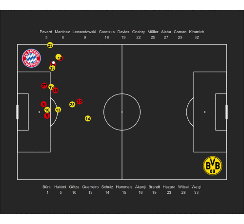
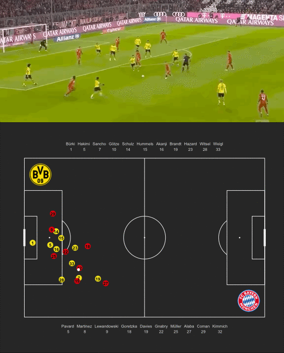
Let’s look at another example that highlights the interpolation step:
In the official footage we can see how the camera zooms in right after Pavard receives the ball. For these few seconds SkillCorner does not provide tracking data as there is not much to track. But we can see that our interpolation does a reasonable job and the movements do not look artificial at all.
I hope this post provides a good starting point to explore this new open-source dataset.
Ressources
- SkillCorner website
- SkillCorner data repository
- Download code for this post
- To not miss any of my future posts, follow me on Twitter